This post is also available on the In Development website.
History remembers two Robert McNamaras.
Lingering in public memory is McNamara as US secretary of defense—the architect of America’s escalation in Vietnam and, for a time, one of the most vilified figures in the country. Then, for a thin slice of development specialists, Robert McNamara is remembered as president of the World Bank. From 1968 to 1981, he led a second war, the war against global poverty, a struggle to which he dedicated extraordinary personal effort—but a war which, for him, ended also in disillusionment.
It is tempting to try and separate the two McNamaras. His tenures at the Pentagon and the World Bank each deserve, and have received, the space of a full-length biography. The two chapters of his life—as head of the “greatest war machine in the history of the world,” then antipoverty crusader—clash like thesis and antithesis.
But, when considered together, the two wars of Robert McNamara’s life reveal a common approach, one that defined the postwar era of global development. Nicknamed “an IBM machine with legs,” McNamara was the living embodiment of midcentury American technocracy—a man who brought an ambitious drive to scale, a rationalizing impulse, and (most of all) a faith in the power of quantification to solve our most pressing social problems.
“To this day,” he wrote near the end of his life, “I see quantification as a language to add precision to reasoning about the world. Of course, it cannot deal with issues of morality, beauty, and love, but it is a powerful tool too often neglected when we seek to overcome poverty, fiscal deficits, or the failure of our national health programs.”
This approach made McNamara’s early career a glittering success. During World War II, he brought statistical control to the US Air Force’s bombing of Japan. At 24, he was made the youngest assistant professor at Harvard Business School. At 44, he became the first person outside the Ford family to preside over the Ford Motor Company—a job he left after just five weeks, to join President John F. Kennedy’s cabinet. At the Pentagon, and then the Bank, he presided over massive increases in spending, bending these huge bureaucracies to his will and reassembling them into their modern forms.
And yet, when the sum total of his career is considered, the overwhelming sense is one of failure. The final years of McNamara’s life were spent reckoning with the wreckage of his legacy.
Where did things go so wrong?
In 1960, the newly elected John F. Kennedy offered McNamara the choice of secretary of the treasury or secretary of defense. McNamara, who claimed to know little about finance, chose defense. Amid the arms race with the Soviet Union, he was now in charge of 9% of all spending in the US economy, and more than half of every federal tax dollar.
His first task was bringing this spending to heel. He introduced the Planning, Programming, and Budgeting System (PPBS), which helped coordinate spending across the army, navy, and air force, and remains the main way the Pentagon allocates funds. With advice from the RAND Corporation, he created a new Office of Systems Analysis, which centered cost-effectiveness as a criterion for spending. It was perhaps the first serious attempt by a civilian to exert control over the Department of Defense—and remains the foundation of defense procurement to this day.
McNamara later said that, had Kennedy not been assassinated, the United States would not have become entangled in Vietnam. Perhaps, then, McNamara might have been remembered by history as a technocratic reformer. But under President Lyndon B. Johnson, McNamara instead became known as one of the fiercest advocates of escalation.
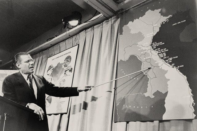
Robert McNamara pointing at a map of Vietnam during a press conference. Photo by Marion S. Trikosko; reproduced from the Library of Congress. As head of the Pentagon, McNamara presided over a massive scale-up in South Vietnam. In 1961, there were still just 3,200 American troops in-country. By 1968, there were over half a million. From 1965 to 1970, they were fed and supplied by 3 million tons of dry goods shipped by sea. (This transpacific traffic would later set off the containerization revolution in global trade.) Overhead, American planes would eventually drop 7.5 million tons of bombs on Vietnam, more than double the amount dropped on Europe and Asia during World War II.
But the Vietnam War was more than just a military conflict. The need to “win hearts and minds” put questions of development at the center of the war—and although South Vietnam ceased to be a country over 50 years ago, it remains the fourth-largest recipient of US foreign aid in history. Perhaps without fully realizing it, McNamara was presiding over a massive, quixotic effort to develop a country that had not asked for it.
The Pentagon’s strategy was informed by a vast new statistical apparatus, the Hamlet Evaluation System. Starting in 1967, every month, an army of surveyors canvassed 12,000 hamlets (subunits of villages) in an active warzone. Hamlets were graded on a scale from “A” for friendly to “E” for contested, based on recorded attacks by Viet Cong or North Vietnamese forces. Alongside the wartime metrics were a host of other variables: questions about levels of education, the state of public works, conditions in agriculture.
Each month, the data from the Hamlet Evaluation System would be fed into an IBM 1410, which would spit out time-series plots that invariably showed that the US was winning the war. Another grisly statistic, the crossover point, measured the juncture at which more North Vietnamese and Viet Cong were being killed than could be replaced. Yet despite the mounting body counts, the tons of bombs dropped, and the purported success of pacification schemes, the North Vietnamese showed little interest in coming to the bargaining table.
The problem, McNamara’s critics stated at the time, was mistaking the war as something that could be understood as a purely quantitative exercise. Counting enemy casualties or pacified villages measured what was legible at the expense of what was strategically important. The North Vietnamese proved willing to absorb losses that American planners did not anticipate. By contrast, fundamental reform to address the root causes of why the Vietnamese were fighting—such as land reform to benefit peasant farmers—was delayed until it was too late.
Archival evidence suggests that McNamara had realized as early as November 1965 that the war could not be won—just months after he had pushed for massive escalation. Within the closed doors of the Johnson administration, he began advocating for a negotiated peace. Quietly, he also assembled a team of analysts, including the economist Daniel Ellsberg, to compile a set of secret papers on the errors of judgment that had led to American involvement.
Yet, for almost two years, McNamara continued to go out and sell the war to the American people. In November 1966, he told the press that “military victory [for the North Vietnamese and Viet Cong] is beyond their grasp.” In 1968, in a statement to the Senate Armed Services Committee, he claimed the Government of South Vietnam was making “encouraging progress.”
The cost of McNamara’s silence was enormous. Although precise estimates are impossible, perhaps 100,000 to 150,000 Vietnamese civilians were being killed each year. From 1965 to 1968, American deaths averaged over 9,100 a year. Decades later, landmines planted during the war were still mutilating children. The carcinogen Agent Orange—sprayed wantonly over fields and villages—is estimated to have caused another 400,000 excess deaths.
When pressed years later on why he had remained silent, McNamara responded with the limp excuse that his ultimate loyalty lay with the president. (Notably, Cabinet secretaries swear their oath of office to defend the Constitution, not the president.) Perhaps he also believed that he could still influence the administration’s policy from the inside. For McNamara, the consummate system builder, it was impossible to imagine himself on the outside.
Privately, the cost of continuing the lie exerted a psychic toll. At night, McNamara ground his molars down to stumps, forcing a painful dental operation. His college-aged son and daughter turned against him. The tension between the sunny and confident public McNamara, and the haunted and doubt-ridden private one, was unsustainable.
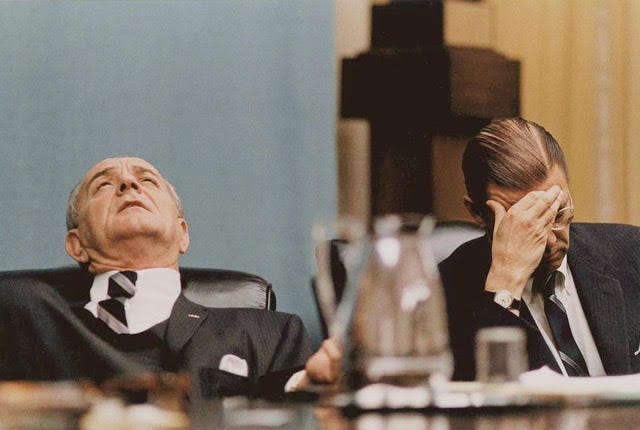
President Lyndon B. Johnson and McNamara in the Cabinet Room in 1968. Photo courtesy of the National Archives. At the end of 1967, President Johnson announced that he was nominating McNamara to be president of the World Bank. Johnson had grown tired of McNamara’s doubts; McNamara, having reportedly suffered a mental breakdown, took the offer. Years later, he recalled telling his friend Katharine Graham, the publisher of The Washington Post, that he didn’t know if he quit or was fired.
“You’re out of your mind,” she said. “Of course you were fired.”
Bruised and drained by his final years as secretary of defense, McNamara found new vitality in the task of remaking the World Bank.
The Bank in 1968 was riddled with contradictions. It had been created to support the postwar rebuilding of Europe, but had been largely bypassed by the United States in favor of the Marshall Plan. It had pivoted to lending to developing countries (starting with a loan to Chile in 1948), but it still depended on capital from Wall Street, whose conservatism chafed at the risks of lending to poor countries. The result was a portfolio that was, in McNamara’s words, “small and patchy”—around $10 billion in today’s dollars, compared to the current portfolio of $120 billion. Moreover, the Bank had no central accounting system, no processes in place to evaluate the impacts of its lending, and no systematic projections of its loan portfolio. According to McNamara, a culture of “leisurely perfectionism” prevailed at the Bank; the process for finalizing projects was slowed by unnecessary technical reviews, and deadlines often slipped.
For a man of McNamara’s ambitions, this was unacceptable. He worked 12-hour days, divided meticulously into 15-minute blocks. He traveled constantly to the developing world, and made a point of venturing outside of capital cities and boardrooms, to see what the living conditions of the poor were really like. McNamara said little publicly about what drove this frenzy of activity. Any connection with demons from Vietnam must be heard in the silences. But his assistant, Olivier LaFourcade, said that it seemed as if “the emotions of a highly emotional person were subdued, controlled.”
Just as he had at the Pentagon, McNamara first sought to exert centralized control over the Bank’s sprawling operations. He ordered the Bank’s senior managers to draw up standardized tables of its lending, and developed the “country program paper,” a common framework for Bank staff to evaluate member countries. A new Programming and Budget department controlled the allocation of resources within the Bank. In 1970, faced with the looming threat of a US Congressional audit, he created the Operations Evaluation Unit to monitor the performance of the Bank’s loans. In 1973, Bank management even pushed to measure the “social rate of return” of development projects. Staff resisted, and the change was scrapped.
Having consolidated his power within the Bank, McNamara next brought his relentless drive to scaling operations. He grew the Bank’s staff more than threefold, from 1,600 employees to 5,700, and began hiring economics graduates from the top American and European schools, transforming the Bank from an institution run by engineers to one dominated by economists. He canvassed Europe, Asia, and the Middle East, expanding the Bank’s pool of creditors beyond Wall Street. He brought on the talented financier Eugene Rotberg, who invented the world’s first currency swap to facilitate the Bank’s borrowing. In total, over McNamara’s presidency, the Bank’s yearly lending grew from around $1 billion in 1968 to $13 billion in 1981—an annualized growth rate of 20%, a pace which no other World Bank president has matched.
There were growing pains. McNamara’s focus on hitting lending targets created incentives to push money out the door, with, Nancy Birdsall notes, “relatively little regard for how it would be used.” To avoid missing targets, loans “bunched” up around key reporting deadlines, a phenomenon that persists at the Bank. A decade later, an internal audit of the Bank found evidence of an “approval culture,” which, ex ante, was overly optimistic about projects’ prospects and, ex post, did little to assess their outcomes.
But the positive imprint McNamara left on the Bank also cannot be denied. The skills he had once applied to the escalation of Vietnam—the drive to scale, the bureaucratic command, the impulse to rationalize and quantify—found a productive new quarry in the struggle for global development. Indeed, during McNamara’s early Bank presidency, aid became central to growth in a way it has not been before or since. In 1970, official development assistance was responsible for 10% of investment in low- and middle-income countries (LMICs), and 16% of their imports. By comparison, in 2021, aid accounted for just 2% of investment and 3% of imports in LMICs.
By the 1970s, however, it was clear that growth was not having the expected effects on poverty throughout the developing world. Despite progress in capital accumulation and infrastructure, the benefits were simply not flowing down to the world’s poorest. A 1972 report by the International Labour Organization described unemployment as “chronic and intractable in nearly every developing country… and will not be cured simply by accelerating the rate of growth.”
In a landmark speech at the 1973 annual meeting of the World Bank and International Monetary Fund (IMF) in Nairobi, McNamara announced a new course. He called for a focus on what he called absolute poverty—“a condition of life so degraded by disease, illiteracy, malnutrition, and squalor as to deny its victims basic human necessities.” The narrow focus on “growth of GNP [gross national product]” missed central questions of inequality and distribution; the Bank must take “action… which will directly benefit the poorest.” Notably, McNamara called for tenancy and land reform—policies he had resisted in Vietnam—arguing that an “increasingly inequitable situation will pose a growing threat to political stability.”
Outside events accelerated the Bank’s turn toward global poverty. The 1973 OPEC crisis sent commodity prices soaring, encouraging commodity producers to demand fairer terms of trade and resource sovereignty. In May 1974, a special session of the UN General Assembly spearheaded by developing countries declared a New International Economic Order (NIEO), demanding technology transfers from the rich world, debt relief, and the reform of international institutions like the Bank and the IMF. In December, a subsequent vote for a new Charter of Economic Rights and Duties of States was 120 in favor and 6 against, with 10 abstentions. Every single developing country voted in favor. The 6 against were the United States, the UK, West Germany, Luxembourg, Belgium, and Denmark.
The NIEO represented a major challenge to the US-led international order. McNamara was sympathetic to its arguments—to a point. His moral commitment to the global poor was genuine. But he refused to advocate for deep structural reforms, such as those that might have increased the representation of poor countries at the Bank. With his close ties to the Washington DC political establishment, McNamara generally refused to buck Administration policy—by his own admission, “the US treated the Bank as though it were a US institution.” Modern econometric research suggests that countries that were diplomatically aligned with the US benefited from faster disbursement of loans and looser conditions.
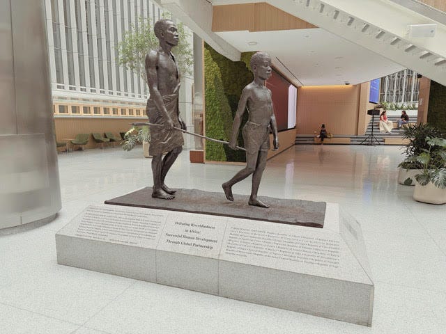
The Bank’s new focus on the global poor produced some notable successes. River blindness, a disease caused by the parasitic worm Onchocerca volvulus, was virtually eradicated thanks to a Bank program with the World Health Organization—by 2002, around 600,000 cases of blindness had been prevented, largely in West Africa. A bronze statue in the World Bank atrium, of a child leading a blind man, marks the achievement.
A statue at the World Bank headquarters symbolizes the collaborative effort to combat river blindness. Photo by Karol Karpinski. But, in the late 1970s, the same structural force that had motivated the Bank’s antipoverty turn—the global rise in commodity prices—began to undermine it. With most developing countries net importers of oil, rising prices forced them to take on debt to finance spending. To address this unfolding crisis, in 1979, McNamara introduced a new lending vehicle, the structural adjustment loan, intended to shore up a government’s general finances rather than support a specific project. In exchange, borrower countries were required to implement macroeconomic reforms: cutting government spending, opening up to trade, and liberalizing the domestic economy.
These first structural adjustment loans—$55 million to Kenya and $200 million to Turkey in 1980—marked the start of the Bank’s departure from the postwar recipe of state-led growth. Over the 1980s and 1990s, this would coalesce into what became known as the Washington Consensus—a mix of market-oriented reforms that emphasized fiscal discipline, liberalization, and the retreat of the state from active economic management.
The economic legacy of this period remains deeply contested. On the one hand, William Easterly finds no evidence of a relationship between structural adjustment loans and better policies or faster growth—perhaps because many of the reforms were never actually undertaken. On the other, defenders of the Consensus point to faster long-run GDP growth among reformers in the 2000s. Outside of economics, public health research suggests that structural adjustment programs, when implemented, led to declines in child and maternal health, likely from cuts to social spending—although this finding is controversial. Separating the effects of structural adjustment from the economic crises that led to those conditions being imposed may simply be an intractable question.
Whatever their precise economic effect, the structural adjustment loans were seen as an expression of the imbalance of power between rich lenders and poor borrowers—precisely the asymmetry that the New International Economic Order had tried to correct.
Moreover, the World Bank’s conditions became publicly associated with the economic disappointment of the 1980s and 1990s. With the afterglow of independence fading, sub-Saharan Africa fell into political instability and economic decline. Growth in Latin America stalled and even reversed amid a wave of debt crises. Morale at the Bank reached a low ebb. McNamara’s dream of a world without poverty, expressed so vividly in Nairobi in 1973, had been perverted beyond recognition. He resigned in 1981, a few months after the death of his wife.
After the World Bank, the last third of McNamara’s life was dominated by trying to confront the ghosts of Vietnam. He read widely, traveled extensively. In 1995, he even went to Hanoi, where he dined with his former North Vietnamese adversaries. (They almost came to blows.)
McNamara’s 1995 biography, In Retrospect, was his first public attempt to come to terms with the past. The book, which is almost entirely about Vietnam, begins with McNamara’s admission that “we were wrong, terribly wrong,” then chronicles the errors of judgment that led America into a quagmire. It makes little mention of his time at the Bank.
In Retrospect was widely panned. For longtime critics of the Vietnam War, it was too little, too late. In his review for the Los Angeles Times, David Halberstam wrote:
Had it been published 25 years ago while the battle itself and the debate over it was still raging—had McNamara come forth then and said, as he does here, that what had come to be known as “McNamara’s War” was “wrong, terribly wrong,” it would have been an extremely valuable part of the ongoing debate; indeed, it might have ended the debate then and there. A secretary of defense of his seeming certitude who came forward and said that he had been mistaken in his earlier estimates and that the war could not be won would have been the most powerful of witnesses...
McNamara’s second attempt to confront his place in history, the 2003 Errol Morris film The Fog of War, was better-received.
Then eighty-five, his face as wrinkled as an almond, McNamara stares directly into the camera and speaks with a crisp lucidity that belies his age. As a byway to Vietnam, he recounts his days in the air force during World War II, when he advised General Curtis LeMay on the firebombing of Tokyo—an operation, he admits, in which they were “behaving as war criminals.” He describes the 13 days of the Cuban Missile Crisis as one of the central American decision-makers, when the world came to the brink of nuclear war. The lesson flashes by in a title card: “rationality alone will not save us.”
And yet that message seemed to elude McNamara, even toward the end of his life. If there is a thread we can trace through his career, from the Pentagon to the Bank, it is that no amount of technocratic skill can substitute for ethical judgment. McNamara was one of the 20th century’s great systems builders—a man who could tame vast bureaucracies, enlarge them, rationalize them. That doing what was right might require sometimes stepping outside the system simply did not compute.
Even after McNamara was forced out by Lyndon Johnson, he refused to publicly come out against Vietnam, repeating the justification that former secretaries of defense should not contradict sitting presidents. At a 2004 event at Berkeley promoting The Fog of War, with the United States entangled in two more foreign wars, McNamara refused to criticize the Bush administration, citing the same principle.
When asked by Errol Morris if he felt responsible for Vietnam, McNamara refused to answer.
“Is it the feeling that you’re damned if you do, and if you don’t, no matter what?” asked Morris.
“Yeah, that’s right,” McNamara said. “And I’d rather be damned if I don’t.”
But one thing stood out to me on rewatching The Fog of War. Notice how quick McNamara is with his figures, particularly those marking human life. He remembers that Allied bombing destroyed 58% of Yokohama, 51% of Tokyo, 99% of Toyama. When asked, he can recite that 25,000 were killed in Vietnam by the end of his tenure at the Pentagon—“just under half,” he points out, of the 58,000 who eventually died.
But also see the pride on his face when he points out that introducing seatbelts at Ford saved 20,000 lives a year. Or when he notes the thirteen years he spent at the World Bank (compared to seven at Defense) working on global poverty.
Perhaps he hoped that there was still a way to make the figures square, to at least net out some of the red. McNamara, who died six years later, was beholden to the numbers to the end.
Oliver Kim is a development economist working as a Research Fellow on Coefficient Giving’s Global Growth Fund. He writes a Substack called Global Developments.
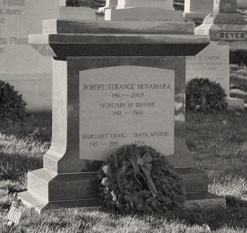
Robert McNamara’s grave in Arlington National Cemetery. Photo by Tim Evanson; CC BY-SA. If you have comments on this article, or wish to contribute to the discussion, please email them to <a href="mailto:letters@indevelopmentmag.com">letters@indevelopmentmag.com</a>. Responses will be featured in a letters section.


